Animated plots using R

I learned the simple concept of animation back in school, when some of my classmates would draw stick figures on the edge of large textbooks. At first I was wondering why one would defile a textbook in such a way, but then as they flipped through the pages and brought the stick figures to life, I was in awe. Despite this, at that stage of my life, a textbook was sacred to me (they were expensive and scarce), so I would use large Post-it notes to doodle instead. I wasn't very good at drawing (even when it comes to stick figures), so I made a few animations and that was it.

This post is on creating animated plots using R. I wrote it not because I wanted to rekindle my youthful interest in stick figure animation but because I wanted to create an animated plot for an upcoming talk. I found a short post on creating animated plots using R and I follow the same idea of making multiple plots and then combining them into a GIF using ImageMagick.

#number of frames or plots
frames <- 50

# function for creating file name with leading zeros
# makes it easier to process them sequentially
rename <- function(x){
  if (x < 10) {
    return(name <- paste('000',i,'plot.png',sep=''))
  }
  if (x < 100 && i >= 10) {
    return(name <- paste('00',i,'plot.png', sep=''))
  }
  if (x >= 100) {
    return(name <- paste('0', i,'plot.png', sep=''))
  }
}

#loop through plots
for(i in 1:frames){
  name <- rename(i)
  
  #saves the plot as a .png file in the working directory
  png(name)
  sd <- 10
  n  <- 10000
  factor <- i * 2
  m  <- 50 + factor
  x  <- rnorm(n, m, sd)
  hist(x,
       xlim=c(0,200),
       ylim=c(0,2000),
       main = paste('Histogram of rnorm() n = ', n, ' mean = ', m, ' sd = ', sd),
       )
  dev.off()
}

#run ImageMagick
my_command <- 'convert *.png -delay 3 -loop 0 animation.gif'
system(my_command)

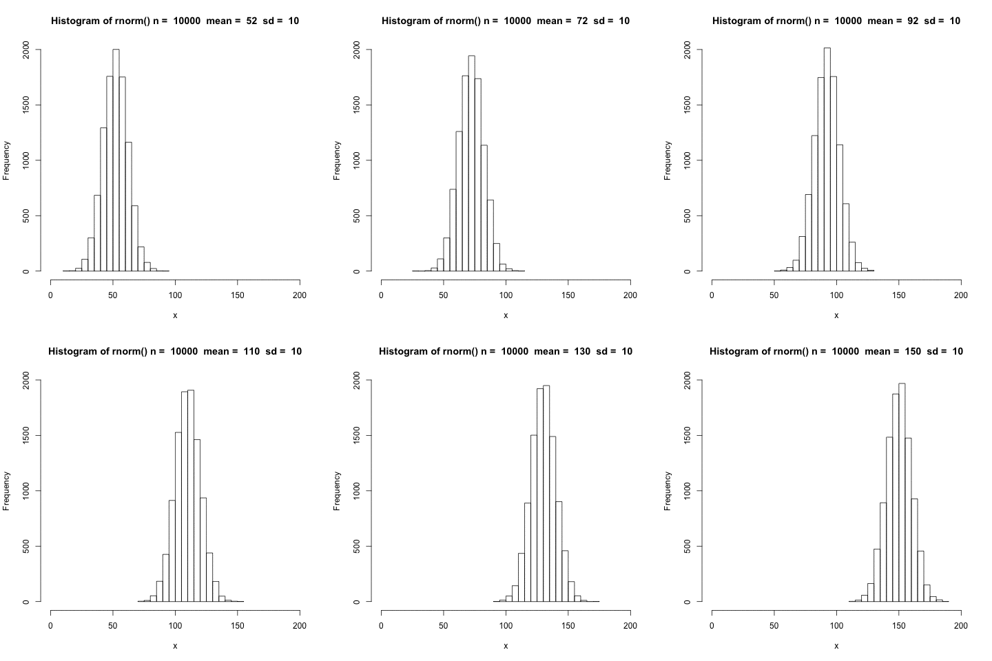
The distribution shifts according to the mean.

Visualise filtering threshold

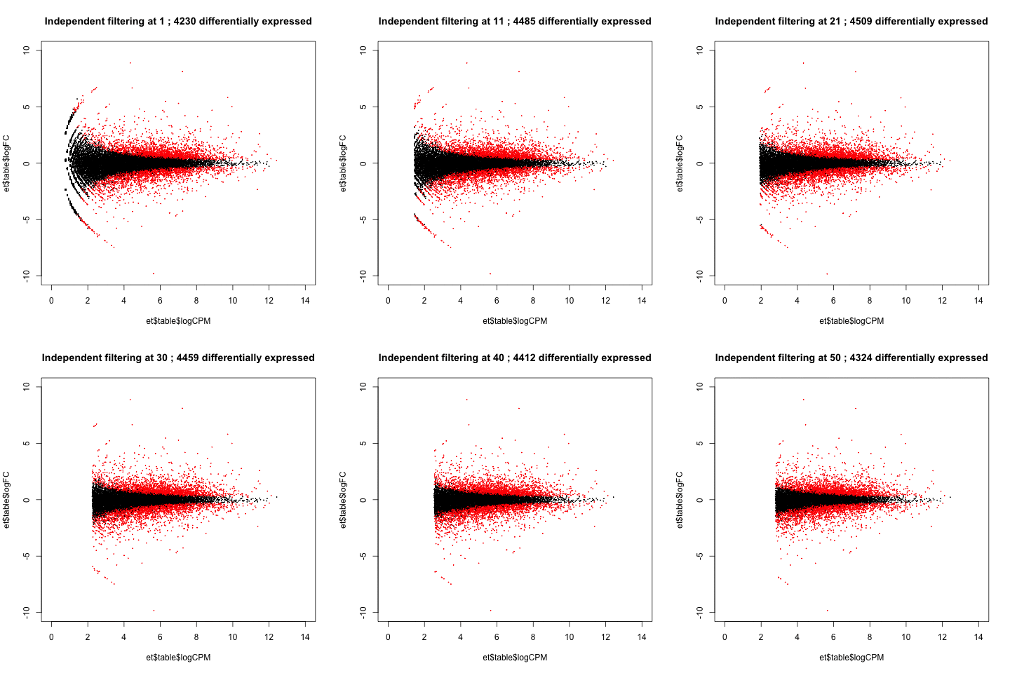
A practical use of animated plots could be to visualise the effects of independent filtering on the number of genes detected as differentially expressed.

frames <- 50
rename <- function(x){
  if (x < 10) {
    return(name <- paste('000',i,'plot.png',sep=''))
  }
  if (x < 100 && i >= 10) {
    return(name <- paste('00',i,'plot.png', sep=''))
  }
  if (x >= 100) {
    return(name <- paste('0', i,'plot.png', sep=''))
  }
}

#I host this file on my server for convenience
file_url <- 'http://davetang.org/eg/pnas_expression.txt'
data <- read.table(file_url,
                   header=T,
                   sep="\t",
                   stringsAsFactors=F,
                   row.names=1
                   )

#remove length column
data <- data[,-8]

library(edgeR)

#loop through plots
for(i in 1:frames){
  name <- rename(i)
  
  #saves the plot as a .png file in the working directory
  png(name)
  data_subset <- subset(data, rowSums(data)>i)
  group <- c(rep("Control",4), rep("Test",3))
  d <- DGEList(counts = data_subset, group=group)
  #data normalisation
  d <- calcNormFactors(d, method="TMM")
  d <- estimateDisp(d)
  et <- exactTest(d)
  de <- table(p.adjust(et$table$PValue, method = "BH")<0.05)[2]
  
  plot(et$table$logCPM,
       et$table$logFC,
       ylim=c(-10,10),
       xlim=c(0,14),
       pch=19,
       cex=0.1,
       col=as.numeric(p.adjust(et$table$PValue, method = "BH")<0.05)+1,
       main=paste("Independent filtering at", i, ';', de, 'differentially expressed')
       )
  dev.off()
}

#run ImageMagick
#I slowed it down a bit more
my_command <- 'convert *.png -delay 5 -loop 0 filtering.gif'
system(my_command)

Adjusting the filtering threshold did not have a large effect on the number of differentially expressed genes. (This isn't always the case.)

Rotating 3D scatter plot

#install.packages("scatterplot3d")
library(scatterplot3d)

data(iris)
frames <- 360

rename <- function(x){
  if (x < 10) {
    return(name <- paste('000',i,'plot.png',sep=''))
  }
  if (x < 100 && i >= 10) {
    return(name <- paste('00',i,'plot.png', sep=''))
  }
  if (x >= 100) {
    return(name <- paste('0', i,'plot.png', sep=''))
  }
}

p <- prcomp(iris[,1:4])
my_col <- as.numeric(iris$Species)

#loop through plots
for(i in 1:frames){
  name <- rename(i)
  
  #saves the plot as a .png file in the working directory
  png(name)
  scatterplot3d(p$x[,1:3],
                main=paste("Angle", i),
                angle=i,
                pch=19,
                cex.symbols=0.5,
                color=my_col)
  dev.off()
}

my_command <- 'convert *.png -delay 1 -loop 0 3d.gif'
system(my_command)

Visualising the three principal components using a 3D scatter plot.

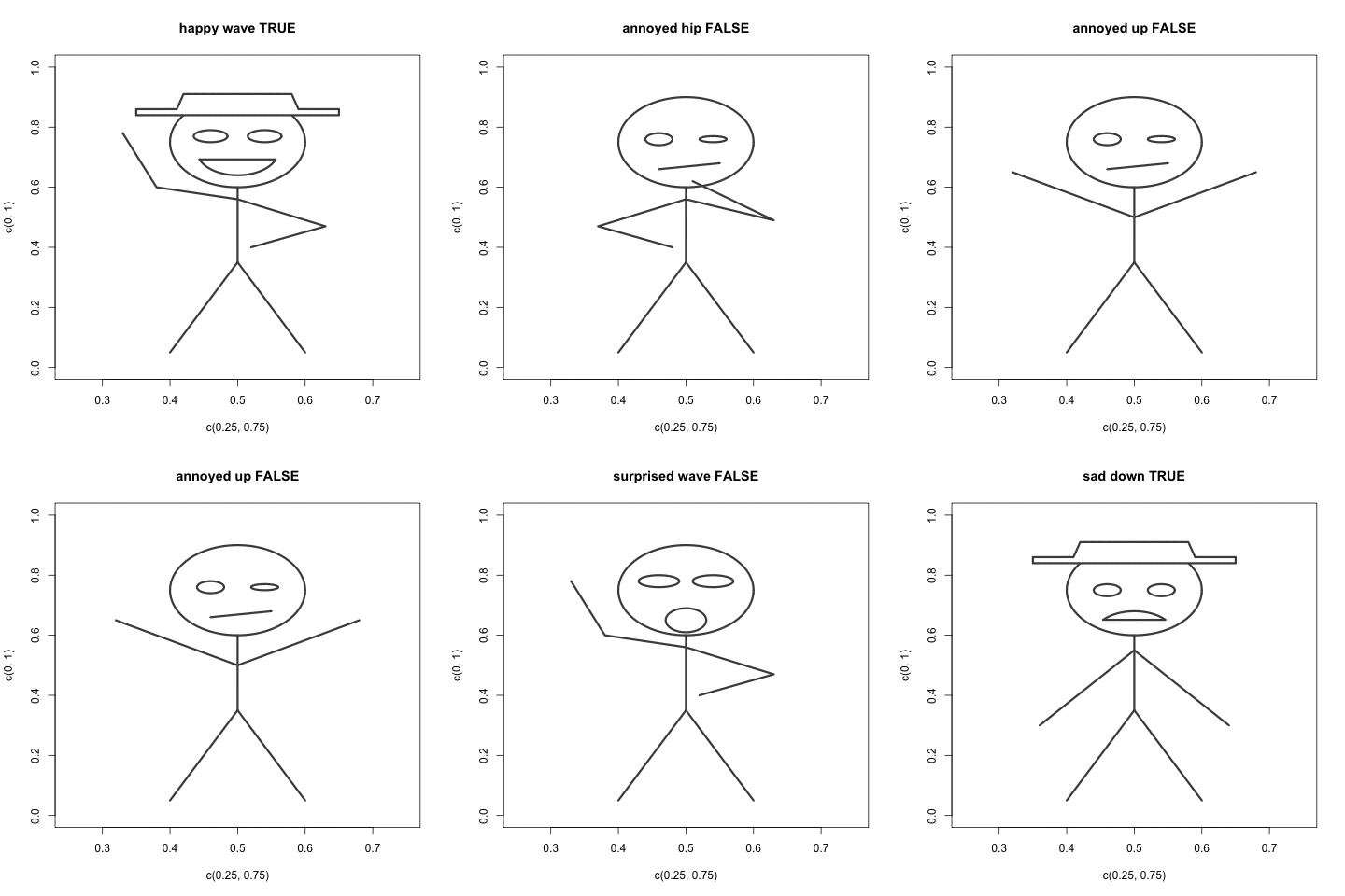
Stick figures

# the XKCD package has a more flexible function for creating stick figures but perhaps for another day
# this draw.stick function is from
# https://github.com/EconometricsBySimulation/R-Graphics/blob/master/Stick-Figures/draw.stick.R
# Stick Man/Woman Generating Function

draw.stick <- function(x,y,scale=1,arms="down", 
                       gender="male",lwd=3, clcol="white",
                       face="happy", linecol=gray(.3),
                       hat=NA) {
  # clcol: color of clothes - any color
  # scale: fize of figure
  # x,y left bottom alignment of figure
  # linecol: color of lines - any color
  # lwd: line weight
  
  # Arms: "down", "neutral", "up", "hip", "wave"
  # Gender: "male", "female"
  # Face: "happy", "sad", "annoyed", "surprised"
  # Hat: plot hat T,F
  
  # Set the figure scale, default it 1
  s <- scale/100
  
  # If is undefined then give the man a hat
  if (is.na(hat)) hat<-(gender=="male")
  
  require("plotrix")
  
  # Draw Head
  draw.ellipse(x+50*s,y+75*s,10*s,15*s,lwd=lwd, border=linecol)
  
  if (face=="happy") {
    # Draw eyes
    draw.ellipse(x+46*s,y+77*s,2.5*s,2*s,lwd=lwd, border=linecol)
    draw.ellipse(x+54*s,y+77*s,2.5*s,2*s,lwd=lwd, border=linecol)
    
    # Draw mouth
    draw.ellipse(x+50*s,y+72*s,6*s,8*s, segment = c(-160,-20),
                 lwd=lwd, border=linecol)
  }
  if (face=="sad")   {
    # Draw eyes
    draw.ellipse(x+46*s,y+75*s,2*s,2*s,lwd=lwd, border=linecol)
    draw.ellipse(x+54*s,y+75*s,2*s,2*s,lwd=lwd, border=linecol)
    
    # Draw mouth
    draw.ellipse(x+50*s,y+60*s,6*s,8*s, segment = c(140,40),
                 lwd=lwd, border=linecol)
  }
  
  if (face=="surprised")   {
    # Draw eyes
    draw.ellipse(x+46*s,y+78*s,3*s,2*s,lwd=lwd, border=linecol)
    draw.ellipse(x+54*s,y+78*s,3*s,2*s,lwd=lwd, border=linecol)
    
    # Draw irises
    #  draw.ellipse(x+46*s,y+78*s,1*s,1*s,lwd=lwd, border=linecol)
    #  draw.ellipse(x+54*s,y+78*s,1*s,1*s,lwd=lwd, border=linecol)
    
    # Draw mouth
    draw.ellipse(x+50*s,y+65*s,3*s,4*s,
                 lwd=lwd, border=linecol)
  }
  
  if (face=="annoyed")  {
    # Draw mouth
    lines(c(x+46*s,x+55*s), c(y+66*s,y+68*s),lwd=lwd, col=linecol)
    
    # Draw eyes
    draw.ellipse(x+46*s,y+76*s,2*s,2*s,lwd=lwd, border=linecol)
    draw.ellipse(x+54*s,y+76*s,2*s,1*s,lwd=lwd, border=linecol)
  }
  
  # Draw torso
  lines(c(x+50*s,x+50*s), c(y+35*s,y+60*s),lwd=lwd, col=linecol)
  
  # Draw arms
  if (arms=="down") {
    lines(c(x+50*s,x+36*s), c(y+55*s,y+30*s),lwd=lwd, col=linecol) # Left
    lines(c(x+50*s,x+64*s), c(y+55*s,y+30*s),lwd=lwd, col=linecol) # Right
  }  
  if (arms=="neutral") {
    lines(c(x+50*s,x+30*s), c(y+50*s,y+55*s),lwd=lwd, col=linecol) # Left
    lines(c(x+50*s,x+70*s), c(y+50*s,y+55*s),lwd=lwd, col=linecol) # Right
  }
  if (arms=="up") {
    lines(c(x+50*s,x+32*s), c(y+50*s,y+65*s),lwd=lwd, col=linecol) # Left
    lines(c(x+50*s,x+68*s), c(y+50*s,y+65*s),lwd=lwd, col=linecol) # Right
  }
  if (arms=="hip") {
    lines(c(x+50*s,x+37*s,x+48*s), c(y+56*s,y+47*s,y+40*s),lwd=lwd, col=linecol) # Left
    lines(c(x+50*s,x+63*s,x+51*s), c(y+56*s,y+49*s,y+62*s),lwd=lwd, col=linecol) # Right
  }
  if (arms=="wave") {
    lines(c(x+50*s,x+38*s,x+33*s), c(y+56*s,y+60*s,y+78*s),lwd=lwd, col=linecol) # Left
    lines(c(x+50*s,x+63*s,x+52*s), c(y+56*s,y+47*s,y+40*s),lwd=lwd, col=linecol) # Right
  }
  
  # Draw male legs
  if (gender=="male") {
    lines(c(x+50*s,x+40*s), c(y+35*s,y+5*s),lwd=lwd, col=linecol)
    lines(c(x+50*s,x+60*s), c(y+35*s,y+5*s),lwd=lwd, col=linecol)
  }
  
  # Draw female legs and dress
  if (gender!="male") {
    # Draw legs
    lines(c(x+45*s,x+45*s), c(y+17*s,y+5*s),lwd=lwd, col=linecol)
    lines(c(x+55*s,x+55*s), c(y+17*s,y+5*s),lwd=lwd, col=linecol)
    
    # Draw dress
    polygon(c(x+s*50,x+s*35,x+s*65), 
            c(y+s*40,y+s*17,y+s*17), 
            col=clcol, border=linecol,lwd=lwd)
  }
  
  # Draw hat
  if (hat==T) polygon(
    c(x+35*s,x+65*s,x+65*s,x+59*s,x+58*s,x+42*s,x+41*s,x+35*s),
    c(y+84*s,y+84*s,y+86*s,y+86*s,y+91*s,y+91*s,y+86*s,y+86*s),
    col=clcol, border=linecol,lwd=lwd)
}

frames <- 50
rename <- function(x){
  if (x < 10) {
    return(name <- paste('000',i,'plot.png',sep=''))
  }
  if (x < 100 && i >= 10) {
    return(name <- paste('00',i,'plot.png', sep=''))
  }
  if (x >= 100) {
    return(name <- paste('0', i,'plot.png', sep=''))
  }
}

#loop through plots
for(i in 1:frames){
  name <- rename(i)
  
  #saves the plot as a .png file in the working directory
  png(name)
  # Arms: "down", "neutral", "up", "hip", "wave"
  # Gender: "male", "female"
  # Face: "happy", "sad", "annoyed", "surprised"
  # Hat: plot hat T,F
  
  a <- c('down','neutral','up','hip','wave')
  f <- c('happy','sad','annoyed','surprised')
  h <- c(TRUE,FALSE)
  fs <- sample(f,1)
  as <- sample(a,1)
  hs <- sample(h,1)
  plot(c(.25,.75),
       c(0,1),
       type="n",
       main=paste(fs, as, hs)
       )
  draw.stick(0,0, face=fs, gender="male", arms=as, hat=hs)

  dev.off()
}

#run ImageMagick
my_command <- 'convert *.png -delay 5 -loop 0 stick_figure.gif'
system(my_command)

The real motivation for this post.