Last updated: 2022 December 12th
On Wikipedia, linear regression is described as:
In statistics, linear regression is a linear approach for modelling the relationship between a scalar response and one or more explanatory variables (also known as dependent and independent variables). The case of one explanatory variable is called simple linear regression; for more than one, the process is called multiple linear regression.
Linear simply means a straight-line, regression in this context means relationship, and modelling means fitting. Therefore, linear regression can be interpreted as trying to find the equation of the straight-line that fits the data points the best and captures the relationship between the variables; the best line is the one that minimises the sum of squared residuals of the linear regression model. The equation of a straight line is:
where $latex m $ is the slope or gradient and $latex b $ is the y-intercept.
Here's a quick example using the "women" dataset that comes with R.
# install the packages below if you haven't already
install.packages('ggplot2')

# load libraries
library(ggplot2)

# check out the data frame
head(women)
#   height weight
# 1     58    115
# 2     59    117
# 3     60    120
# 4     61    123
# 5     62    126
# 6     63    129

# plot height vs. weight
# and fit a linear model
ggplot(women, aes(height, weight)) +
  geom_point() +
  geom_smooth(method = "lm")
There seems to be a relationship between height and weight.
How do we figure out this line of best fit manually? We can work out $latex m $ for the women dataset using this formula:
$latex m = \frac{\sum_{i=1}^{n}(x_i - \overline{x})(y_i - \overline{y})}{\sum_{i=1}^{n}(x_i - \overline{x})^2} &s=4$
where $latex n $ is the number of observations in our dataset, $latex \sum_{i=1}^n $ means the sum all the observations, $latex x_i $ and $latex y_i $ are the $latex i $th observation of $latex x $ and $latex y $, and $latex \overline{x} $ and $latex \overline{y} $ are the means of $latex x $ and $latex y $, respectively.
Once we have $latex m $, we can work out $latex b $ with:
$latex b = \overline{y} - m\overline{x}&s=3 $
which is just a rearrangement of:
but using the mean values.
We can express these functions in R as:
slope <- function(x, y){
  mean_x <- mean(x)
  mean_y <- mean(y)
  nom <- sum((x - mean_x)*(y-mean_y))
  denom <- sum((x - mean_x)^2)
  m <- nom / denom
  return(m)
}

# the slope formula is just
# covariance(x, y) / variance(x)
slope2 <- function(x, y){
  return(cov(x, y)/var(x))
}

intercept <- function(x, y, m){
  b <- mean(y) - (m * mean(x))
  return(b)
}
Before we work out $latex m $ and $latex b $, a word on dependent and independent variables. When modelling, we want to work out the dependent variable from an independent variable (or variables). For this post, we would like to work out weight from height, therefore our independent variable is height and dependent variable is weight. It can be the other way around too. When plotting, the independent variable is usually on the x-axis, while the dependent variable is on the y-axis (as I have done above). Now to use our slope() and intercept() functions.
my_slope <- slope(women$height, women$weight)
my_intercept <- intercept(women$height, women$weight, my_slope)

my_slope
# [1] 3.45
my_intercept
# [1] -87.51667

# let's plot this using base R functions
plot(women$height, women$weight, pch=19)

# add the regression line
abline(my_intercept, my_slope)
This plot looks similar to the ggplot2 version without the confidence intervals.
The lm() function (used for fitting linear models) in R can work out the intercept and slope for us (and other things too). The arguments for lm() are a formula and the data; the formula starts with the dependent variable followed by tilde (~) and followed by the independent variable:
fit <- lm(weight ~ height, women)
fit
#
# Call:
# lm(formula = weight ~ height, data = women)
#
# Coefficients:
# (Intercept)       height
#      -87.52         3.45
#

# other values stored in the lm object
names(fit)
#  [1] "coefficients"  "residuals"     "effects"       "rank"          "fitted.values" "assign"        "qr"
#  [8] "df.residual"   "xlevels"       "call"          "terms"         "model"
Note that the coefficients (Intercept) and height are the same as what we calculated manually for the intercept and slope.
The residuals data is the difference between the observed data of the dependent variable and the fitted values. We can plot our observed values against the fitted values to see how well the regression model fits.
plot(women$weight, fit$residuals, pch=19)
abline(h = 0, lty = 2)
The fourth point from the left has a residual that is close to zero; this is because the fitted weight (122.9333 pounds) is almost the same as the real weight (123 pounds) for someone who is 61 inches tall.
We can use the predict() function to predict someone's weight based on their height.
# predict someone's weight when they are 61 inches tall
predict(fit, data.frame(height = 61))
       1
122.9333

# predict someone's weight when they are 80 inches tall
predict(fit, data.frame(height = 80))
       1
188.4833
The example in Statistics for Dummies
There's a nice example on linear regression in the "Statistics For Dummies" book that also demonstrates how you can manually calculate the slope and intercept. Here I'll perform the analysis using R and the data containing the number of cricket (the insect) chirps versus temperature. First we will create the vectors containing the chirps and temperature.
chirp <- c(18,20,21,23,27,30,34,39)
temp <- c(57,60,64,65,68,71,74,77)
The five summaries required for calculating the slope and intercept of the best fitting line are:
- The mean of x
- The mean of y
- The sd of x
- The sd of y
- The r between x and y
We can work out the five summarises using built-in functions in R.
mean(chirp)
# [1] 26.5
mean(temp)
# [1] 67
sd(chirp)
# [1] 7.387248
sd(temp)
# [1] 6.845228
cor(chirp,temp)
# [1] 0.9774791
We can use the third equation in the Wikipedia article to work out the slope.
Note that in the "Statistics For Dummies" book, dependent variables are referred to as response variables and independent variables are referred to as explanatory variables. You can think of the response variable as the variable that responds on a set of variables (explanatory variables) that explains the response.
# formula for the slope m, response variable first
# m = r(sd(x) / sd(y))
m <- cor(chirp,temp) * (sd(chirp)/sd(temp))
m
# [1] 1.054878

# formula for intercept as above
# b = mean(y) - (m * mean(x))
mean(chirp) - (m * mean(temp))
# [1] -44.17683
We can use the lm() function in R to check our calculation. Models for lm() are specified symbolically and a typical model has the form response ~ terms, where response is the response vector and terms is a series of terms which specifies a linear predictor for response.
We'll make chirps the response (dependent variable) and temperature the explanatory variable (independent variable), i.e. predicting the number of chirps from the temperature.
lm(chirp~temp)

# Call:
# lm(formula = x ~ y)
#
# Coefficients:
# (Intercept)            y
#     -44.177        1.055
We see that the coefficients are the same as what we had calculated. We can use the slope and intercept to write a function to predict the number of chirps based on temperature.
# in the form y = mx + b
# y = 1.055x - 44.177
model <- function(x){
   1.055 * x - 44.177
}

# how many chirps at 68 Fahrenheit using our linear model?
model(68)
# [1] 27.563

model(77)
# [1] 37.058
We can check our function using the built-in R function called predict().
reg <- lm(chirp~temp)
predict(reg, data.frame(temp=68))
#        1
# 27.55488

predict(reg, data.frame(temp=77))
#        1
# 37.04878
The linear model generated by R contains some useful information such as the coefficient of determination (i.e. R-square).
summary(reg)$r.squared
# [1] 0.9554655
Use the summary() function to get a full summary.
summary(reg)
#
# Call:
# lm(formula = chirp ~ temp)
#
# Residuals:
#     Min      1Q  Median      3Q     Max
# -2.3354 -0.8872 -0.2195  1.1509  2.0488
#
# Coefficients:
#              Estimate Std. Error t value Pr(>|t|)
# (Intercept) -44.17683    6.25773   -7.06 0.000404 ***
# temp          1.05488    0.09298   11.35 2.81e-05 ***
# ---
# Signif. codes:  0 ‘***’ 0.001 ‘**’ 0.01 ‘*’ 0.05 ‘.’ 0.1 ‘ ’ 1
#
# Residual standard error: 1.684 on 6 degrees of freedom
# Multiple R-squared:  0.9555,  Adjusted R-squared:  0.948
# F-statistic: 128.7 on 1 and 6 DF,  p-value: 2.808e-05
Finally, we can plot the data and add the line of best fit. As per convention, the response variable is on the y-axis and the explanatory variable is on the x-axis
plot(temp, chirp, pch=19)
abline(reg)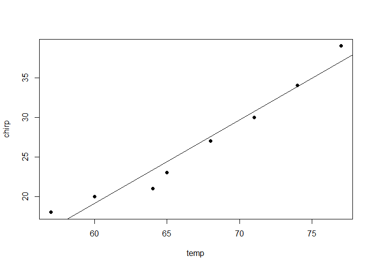
The same plot can be generated using ggplot2.
library(ggplot2)
# response variable on the y-axis
qplot(temp, chirp, geom = c("point", "smooth"), method="lm")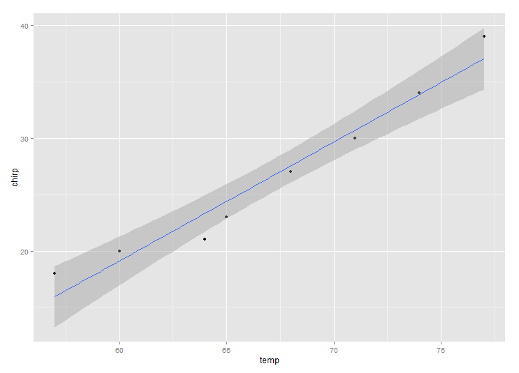


This work is licensed under a Creative Commons
Attribution 4.0 International License.
Your blog is amazing, thank you very much, it’s quite easy to read during stress. I used your blog to come to the realization that given that I was looking for the angle of my line with the x-axis but the regression equation was too far out there, I had to standardize my data to be able to get that angle. I was wondering if maybe you would like to add something link that to this entry. It’s quite useful for analyzing deforestation trends for example, but I don’t see it often because only psycologists seem to use standardization
Hi Pablo,
I’m glad you found the post useful. I didn’t quite follow your comment about adding a link. I’m happy to add a link if it’s relevant and useful.
Cheers,
Dave