For a while, heatmap.2() from the gplots package was my function of choice for creating heatmaps in R. Then I discovered the superheat package, which attracted me because of the side plots. However, shortly afterwards I discovered pheatmap and I have been mainly using it for all my heatmaps (except when I need to interact with the heatmap; for that I use d3heatmap).
The one feature of pheatmap that I like the most is the ability to add annotations to the rows and columns. To get started, you can install pheatmap if you haven't already.
install.packages(pheatmap)

# load package
library(pheatmap)
I will use the same dataset, from the DESeq package, as per my original heatmap post.
# install DESeq if necessary
if (!requireNamespace("BiocManager", quietly = TRUE))
    install.packages("BiocManager")

# install and load package
BiocManager::install("DESeq")
library("DESeq")

# if you can't install DESeq, I have hosted the file at https://davetang.org/file/TagSeqExample.tab
# example_file <- "https://davetang.org/file/TagSeqExample.tab"

# load data and subset
example_file <- system.file ("extra/TagSeqExample.tab", package="DESeq")
data <- read.delim(example_file, header=T, row.names="gene")
data_subset <- as.matrix(data[rowSums(data)>50000,])

# create heatmap using pheatmap
pheatmap(data_subset)

The heatmap.2() function has a parameter for scaling the rows; this can be easily implemented.
cal_z_score <- function(x){
  (x - mean(x)) / sd(x)
}

data_subset_norm <- t(apply(data_subset, 1, cal_z_score))
pheatmap(data_subset_norm)

Now before I demonstrate the main functionality that I like so much about pheatmap, which is creating annotations, we need to figure out how we would like to colour the rows. I'll perform hierarchical clustering in the same manner as performed by pheatmap to obtain gene clusters. I use the excellent dendextend to plot a simple dendrogram.
my_hclust_gene <- hclust(dist(data_subset), method = "complete")

# install if necessary
install.packages("dendextend")

# load package
library(dendextend)

as.dendrogram(my_hclust_gene) %>%
  plot(horiz = TRUE)

We can form two clusters of genes by cutting the tree with the cutree() function; we can either specific the height to cut the tree or the number of clusters we want.
my_gene_col <- cutree(tree = as.dendrogram(my_hclust_gene), k = 2)

my_gene_col
Gene_00562 Gene_02115 Gene_02296 Gene_02420 Gene_02800 Gene_03194 Gene_03450 Gene_03852 Gene_03861 Gene_04164
         1          2          2          2          2          2          2          2          2          2
Gene_05004 Gene_05761 Gene_05960 Gene_06899 Gene_07132 Gene_07390 Gene_07404 Gene_08042 Gene_08576 Gene_08694
         2          2          2          2          2          1          2          1          2          1
Gene_08743 Gene_08819 Gene_09238 Gene_09505 Gene_09610 Gene_09952 Gene_09969 Gene_10648 Gene_10924 Gene_11002
         1          1          1          2          2          2          2          2          2          2
Gene_11672 Gene_12318 Gene_12576 Gene_12804 Gene_12834 Gene_12940 Gene_13444 Gene_13540 Gene_14450 Gene_14672
         1          2          2          1          2          1          2          1          1          1
Gene_14928 Gene_15286 Gene_15334 Gene_16114 Gene_16632 Gene_17743 Gene_17849 Gene_17865 Gene_17992
         2          2          2          1          1          1          2          2          2
The 1's and 2's indicate the cluster that the genes belong to; I will rename them using the ifelse() function and create a data frame, which is the data structure needed by pheatmap for creating annotations.
my_gene_col <- data.frame(cluster = ifelse(test = my_gene_col == 1, yes = "cluster 1", no = "cluster 2"))

head(my_gene_col)
             cluster
Gene_00562 cluster 1
Gene_02115 cluster 2
Gene_02296 cluster 2
Gene_02420 cluster 2
Gene_02800 cluster 2
Gene_03194 cluster 2
We can add multiple row annotations to a heatmap and below I'll add some random annotations.
set.seed(1984)
my_random <- as.factor(sample(x = 1:2, size = nrow(my_gene_col), replace = TRUE))
my_gene_col$random <- my_random

head(my_gene_col)
             cluster random
Gene_00562 cluster 1      2
Gene_02115 cluster 2      1
Gene_02296 cluster 2      1
Gene_02420 cluster 2      1
Gene_02800 cluster 2      2
Gene_03194 cluster 2      2
I'll add some column annotations and create the heatmap.
my_sample_col <- data.frame(sample = rep(c("tumour", "normal"), c(4,2)))
row.names(my_sample_col) <- colnames(data_subset)
my_sample_col
sample
T1a tumour
T1b tumour
T2 tumour
T3 tumour
N1 normal
N2 normal
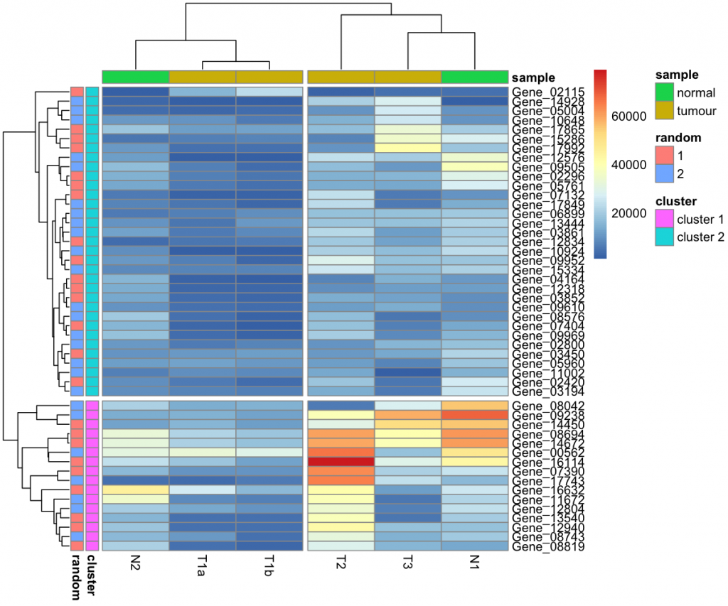
pheatmap(data_subset, annotation_row = my_gene_col, annotation_col = my_sample_col)

Another function that I like about pheatmap is the ability to introduce breaks in the heatmap. I'll break up the heatmap by specifying how many clusters I want from the dendrograms. (You can also manually define where you want breaks too.)
pheatmap(data_subset,
         annotation_row = my_gene_col,
         annotation_col = my_sample_col,
         cutree_rows = 2,
         cutree_cols = 2)

If you want to change the colours, use the annotation_colors parameter.
my_gene_col <- cutree(tree = as.dendrogram(my_hclust_gene), k = 2)
my_gene_col <- data.frame(cluster = ifelse(test = my_gene_col == 1, yes = "cluster1", no = "cluster2"))
my_sample_col <- data.frame(sample = rep(c("tumour", "normal"), c(4,2)))
row.names(my_sample_col) <- colnames(data_subset)

# change order
my_sample_col$sample <- factor(my_sample_col$sample, levels = c("normal", "tumour"))

set.seed(1984)
my_random <- as.factor(sample(x = c("random1", "random2"), size = nrow(my_gene_col), replace = TRUE))
my_gene_col$random <- my_random

my_colour = list(
    sample = c(normal = "#5977ff", tumour = "#f74747"),
    random = c(random1 = "#82ed82", random2 = "#9e82ed"),
    cluster = c(cluster1 = "#e89829", cluster2 = "#cc4ee0")
)

p <- pheatmap(data_subset,
              annotation_colors = my_colour,
              annotation_row = my_gene_col,
              annotation_col = my_sample_col)

Finally, I'll demonstrate how you can retrieve the hierarchical clustering information using pheatmap. (I showed how you can manually perform the same hierarchical clustering as pheatmap in this post but if you didn't, this step is handy.)
# use silent = TRUE to suppress the plot
my_heatmap <- pheatmap(data_subset, silent = TRUE)

# results are stored as a list
class(my_heatmap)
[1] "list"

names(my_heatmap)
[1] "tree_row" "tree_col" "kmeans"   "gtable"

my_heatmap$tree_row %>%
  as.dendrogram() %>%
  plot(horiz = TRUE)

Saving heatmap
To output the heatmap as a PNG file, save the heatmap as an object and use the grid.draw() function on the gtable slot.
library("DESeq")
library("pheatmap")
library("dendextend")

example_file <- system.file ("extra/TagSeqExample.tab", package="DESeq")
data <- read.delim(example_file, header=T, row.names="gene")
data_subset <- as.matrix(data[rowSums(data)>50000,])

cal_z_score <- function(x){
  (x - mean(x)) / sd(x)
}

data_subset_norm <- t(apply(data_subset, 1, cal_z_score))
my_hclust_gene <- hclust(dist(data_subset), method = "complete")
my_gene_col <- cutree(tree = as.dendrogram(my_hclust_gene), k = 2)
my_gene_col <- data.frame(cluster = ifelse(test = my_gene_col == 1, yes = "cluster 1", no = "cluster 2"))
set.seed(1984)
my_random <- as.factor(sample(x = 1:2, size = nrow(my_gene_col), replace = TRUE))
my_gene_col$random <- my_random
my_sample_col <- data.frame(sample = rep(c("tumour", "normal"), c(4,2)))
row.names(my_sample_col) <- colnames(data_subset)
my_heatmap <- pheatmap(data_subset,
                       annotation_row = my_gene_col,
                       annotation_col = my_sample_col,
                       cutree_rows = 2,
                       cutree_cols = 2)

save_pheatmap_png <- function(x, filename, width=1200, height=1000, res = 150) {
  png(filename, width = width, height = height, res = res)
  grid::grid.newpage()
  grid::grid.draw(x$gtable)
  dev.off()
}

save_pheatmap_png(my_heatmap, "my_heatmap.png")
Summary
There are various heatmap packages in R. I like pheatmap mainly because of its annotation feature; other heatmap packages may be able to do the same thing but I'm happy with pheatmap. Use ?pheatmap to find out more ways you can customise your heatmap.


This work is licensed under a Creative Commons
Attribution 4.0 International License.
wow! what a clear and concise explanation! thank you
Great tutorial! You may also want to check out NMF::aheatmap (http://nmf.r-forge.r-project.org/aheatmap.html). It’s a fork of pheatmap with a few additional features / convention changes.
Thanks Keith! I will check it out.
Pheatmap by default creates a new plot. Do you know if there’s any reasonable way to add a pheatmap to a bigger panel? Eg:
> par(mfrow=c(2,2))
> …a graph…
> ..another graph…
> pheatmap(….)
So my pheatmap would now be on the lower left corner of my figure panel. Can this be done from within R or only post-processing?
You can use the gridExtra package. See my other reply: https://davetang.org/muse/2018/05/15/making-a-heatmap-in-r-with-the-pheatmap-package/#comment-8232
When i try to run :
row.names(my_sample_col) <- colnames(CommonUpPvalue)
my_sample_col :
sample
1 tumour
2 tumour
3 tumour
4 tumour
5 normal
6 normal
Error in `.rowNamesDF<-`(x, value = value) : invalid 'row.names' length
any help ?
Hard to say without knowing the structure of CommonUpPvalue.
Thank you for the tutorial.
Do you know how to extract the height values for each sample as they are plotted in the dendrogram?
You can extract the heights from the hclust object.
Hi Dave I fell at the 2nd hurdle of making the z score
> cal_z_score mat_norm pheatmap(mat_norm)
Error in hclust(d, method = method) :
NA/NaN/Inf in foreign function call (arg 11)
any ideas why?
I am also receiving this same error. Was there a solution posted?
Thanks
Are you running the example code on this post or something else? I just ran the following and had no problems.
library(DESeq) example_file <- system.file ("extra/TagSeqExample.tab", package="DESeq") data <- read.delim(example_file, header=T, row.names="gene") data_subset <- as.matrix(data[rowSums(data)>50000,]) cal_z_score <- function(x){ (x - mean(x)) / sd(x) } data_subset_norm <- t(apply(data_subset, 1, cal_z_score)) pheatmap(data_subset_norm)Hi Dave,
That’s a beautiful tutorial. Do you happen to know how to group multiple pheatmaps on the same page.? For instance, I have two pheatmaps saved as dataframes: eraheat and gdfheat. I want to place the two plots together. Can you advise on how to go about this?
Hi there,
you can use the gridExtra package. For example:
Hi Dave,
Simple, clear and complete…
That was excellent tutorial and useful for me.
So much thanks
Hi Dave,
I am looking for the xl file arrangement for this heatmap. Could you please say how can I get it?
Hi there,
if you run the following, you can get the location of the file.
example_file <- system.file ("extra/TagSeqExample.tab", package="DESeq") example_file [1] "/Library/Frameworks/R.framework/Versions/3.6/Resources/library/DESeq/extra/TagSeqExample.tab"Thanks for the grat tutorial!
In my case I have 3 clusters after cutree. How do I transform the data into a data.frame? Can you help me?
For 3 clusters, you can do something like this:
Thanks!!! That worked perfectly.
Hi Dave,
Excellent tutorial, helped me a lot with making a heatmap to color annotation to both rows and columns.
In your tutorial, for scaling a row you calculated Z score but Pheatmap has a “scale” function too. I am just wondering what is the difference between “scale” function in the Pheatmap and Z score. In the Pheatmap manual, the scale is described as a ‘character indicating if the values should be centered and scaled in either the row direction or the column direction, or none. Corresponding values are “row”, “column” and “none”‘.
Hi Ali,
they are the same. I really should just use the scale parameter in pheatmap instead of writing a function. If you want to learn more about scale, type ?scale in R.
Cheers,
Dave
Great example! I was wondering if there is a way to group the samples (columns) based on the factor levels in cluster column you made (i.e. cluster 1, cluster 2) ? it will be similar to the output when kmeans_k != NA.
Hi there! I’m not sure I am following. You want to group the columns using the row groupings?
Hi DAVO,
Thanks for the great tutorial!
In my case, I have 6 clusters after cutree. How do I transform the data for 6 clusters with different colours into a data.frame? Any suggestion would be appreciated.
I created an example with 6 clusters at https://davetang.github.io/muse/pheatmap.html. Please scroll down until you find the section “More clusters.”
Hello Davo,
I have a question about, how to change the order of clusters according to tree (top to bottom) and extract this same in csv file . For example, I want to move cluster 1 to top, cluster 2 in 2nd top, cluster 3 on 3rd, and cluster 6 on the bottom. How can I re-order the position of clusters? Any suggestion.
You can get the order from the dendrogram object and use the match function in R to change the order of your clusters. I’m not sure how you can re-order the heatmap dendrogram using pheatmap. There is probably a way using the ComplexHeatmap package, which uses dendextend to draw the dendrograms.
Thanks, DAVO for your time and help. The examples work perfectly for me.
Hi Dave
Thanks a lot for the tutorial, very helpful! I have heatmaps with many rows of differentially expressed genes and I would like to label only a subset of them, which I suceed doing by creating a character vector of “uninteresting rows” blank (“”). However, because the rows are too narrow, the text label overlaps when the two genes are close in the heatmap. Is there any way to reposition the rowname labels so that they are not overlapping and have a line connecting the repositioned rowname to the original position of that row in the heatmap?
Thanks
Camila
Hi Camila,
I don’t know an easy way to do that! Sorry. It may be easier to export the plot and manually label the rows of interest (though you’ll have to do that again when you generate a new heatmap).
Cheers,
Dave
Dave,
this is awesome ! I have tried our your DESeq2 ttutorial ew years ago and it worked so well. I am revisiting here after years and I saw this pheatmap and wanted to use that on my data matrix . However it is not printing the heatmap at all. i am not getting any error……I just get to the prompt. I am using R studio. Any suggestions as to what I may be missing?
My data is a numerical matrix of 70 by 500 matrix. Any suggestions would be greatly appreciated !
In RStudio, if you are using R Markdown document, the plot should show directly underneath your code (unless you changed the default customisation); take a look at https://davetang.github.io/muse/pheatmap.html. If you are coding in an R Script file, the plot should show in the Plots pane.
Hi Dave,
Nice post !
How do you get the exact order of the genes as plotted in the heatmap.
# cluster the matrix
my_hclust_gene <- hclust(dist(data_subset), method = "complete")
# extract the order of genes from the object my_hclust_gene
data.frame(my_hclust_gene$order, my_hclust_gene$labels)
However, if you visualize the order of genes in data frame, it is different from what is shown in heatmap.
Any suggestions to reorder correctly to get same order from both ways.
thanks !
Hi Chirag,
the order is for data_subset. I updated the code on https://davetang.github.io/muse/pheatmap.html to illustrate; see “Obtaining the gene IDs as per the order of the dendrogram (from top to bottom).”
Cheers,
Dave
Hi Dave,
Thank you for this very useful tutorial. I have been able to implement it successfully. Is there a way to order the columns such that the ‘normal’ tissues are next to each order? I have a situation where two samples (i.e. A & B) were treated and followed over time (i.e. 1, 2 & 3h) and one wishes to view the 3 columns of A corresponding to the time points next to each other, then followed by those of A. Thanks
Hi there,
I have added an example of defining your own column order at https://davetang.github.io/muse/pheatmap.html; scroll down to “Define your own column order…”.
Cheers,
Dave
Thank u Dave! It’s been really helpful!
I have a problem:
I dont want to use R to save the heatmap as a png file.
How can I save the heatmap dataset to process in another Visualization software?
Thank u so much.
Hi there,
I have hosted the dataset used in this blog post at https://davetang.org/file/TagSeqExample.tab.
Cheers,
Dave
Hi Dave,
Is it possible to increase the distance between the main(title) and the dendrogram
Thanks for any comment
Hi Paul,
I have included an example at https://davetang.github.io/muse/pheatmap.html. Please see the section: “Add a title using textGrob; you will need the grid and gridExtra packages.”
Cheers,
Dave
Hello,
Thank you very much for this tutorial. It is very helpful.
I looking to add asterisks on my heatmap (generated whith pheatmap) to show significance level of clustering like for exemple “*” (P value < 0.05) and "**" (P value <0.01).
Is it possible ? Or maybe with some other way than asteriks.
Thank you
Best regards
Hi there,
I don’t know an easy way to achieve that in R. Probably the easiest way is to save the heatmap and then use an image editing program to manually add the asterisks.
Cheers,
Dave
Hello,
Thank tou for your answer. I guess so, I can add the asterisks manually, but how can I get the p-value for each branch ?
Best
RP
Take a look at https://cran.r-project.org/web/packages/pvclust/index.html (and an old post I wrote on using the package https://davetang.org/muse/2010/11/26/hierarchical-clustering-with-p-values-using-spearman/).
Hi David,
Happy New Year!
Thanks for another great post!!
Do you know if there is a way to set break for continues row / col annotation colors? So that the color scale for the same annotation will be the same for different datasets?
Thanks
Siyu
Hi Siyu,
a Happy New Year to you too.
May you provide an example of what you want? Do you want to plot different datasets together in a single heatmap?
Cheers,
Dave
Hi Davo,
thank you for the tutorial. Indeed, it is very helpful for the beginners like me.
I am trying to draw the heatmap for my data. The data is structured in a way that I used the first column as the list of genes the second column is one cancer cell type and the second is another cell type. I tried to structure in a way that you did in the example dataset to avoid confusion.
When i tried to apply the following script I am getting the following errors;
after running the script (my_data <- read.csv("DEGs.tab", package="DESeq")
my_data<- read.delim(my_data, header = T, row.names= "gene")
data_subset 8000,)])
Error in data > 8000 :
comparison (6) is possible only for atomic and list types
when i tried to run the single line of the script, i get this error
Error in read.table(file = file, header = header, sep = sep, quote = quote, :
‘file’ must be a character string or connection
just for your reference, my data structure is like this
gene_name,cell A1, cell A2, cell A3, cell B1, cell b2, cell B3
A,28571.55784,24996.41875,27314.74942,1325.224466,1568.208437,1544.593084
B,17498.06636,15973.18626,15834.70806,2714.557263,2721.211058,2774.343084
C,12421.94019,12034.16958,12768.28879,642.0401563,621.2478017,666.9256713
D,3578.701816,3663.360016,4101.896949,450.6720024,411.0433529,386.7830353
E,3656.475869,3304.687057,3782.762925,343.5058362,314.2660571,365.6242259
F,2674.989236,2579.890959,2797.058447,214.3323324,174.823502,222.5906746
and so on up to line 4414.
Please assist me
Hi there,
you can simply load your data into R by running:
my_data <- read.csv("DEGs.tab", header = TRUE, row.names = "gene_name")Hope that helps,
Dave
Hi Dave,
Can I use the Deseq package for normalized TPM data?
Hi Sanjana,
DESeq (and DESeq2) expects raw counts, so you shouldn’t use normalised data. Try to find the raw data (or you can try to un-normalise data back to its raw state).
Cheers,
Dave
Hi Dave,
I can’t wait to use your wonderful tutorial, but I’m stuck for the beginning.
I have kinda the same problem than MUHAMMAD JAMAL.
I also prepared my table as you did for your example data and also got the same error:
Error in read.table(file = file, header = header, sep = sep, quote = quote, :
‘file’ must be a character string or connection
I tried to change the name of the columns, the name of the gene, without success.
just for your reference, my data structure is like this
Name 110R 41B 1103P 10114 140Ru Rupestris Riapria 420A Berlandieri SO4
Transporter_Transp296 2,50 0,30 0,37 0,19 0,40 2,47 2,79 0,39 0,15 0,43
Fatty Acid_MD-2_10 2,54 0,10 0,00 0,13 0,05 1,83 5,17 0,03 0,11 0,06
Fatty Acid_Lip32 1,71 0,20 0,32 0,26 0,21 2,89 3,21 0,31 0,30 0,59
Thanks for your help,
Cheers
Eldu
Hi Eldu,
the error is from the read.table command and it is saying that you need to provide the name of your file to the command. You need to reformat your table too; the header (first row) does not have commas while the rest of the file uses commas.
Once you modified your file to a comma-delimited file, save it and remember its name and path. Then load it into R as I suggested to Muhammad https://davetang.org/muse/2018/05/15/making-a-heatmap-in-r-with-the-pheatmap-package/#comment-8442.
Hope that helps,
Dave
Hi Dave,
It is a wonderful tutorial I have read. As a biological researcher, it helped me a lot!
I would like to ask for more details about “my_gene_col”.
my_gene_col <- cutree(tree = as.dendrogram(my_hclust_gene), k = 2) # for example k =5
my_gene_col <- data.frame(cluster = ifelse(test = my_gene_col == 1, yes = "cluster 1", no = "cluster 2")) # How to modified the scrpt?
If I want to look up more than 2 clusters, how are the script could be?
Thanks for your help,
Cheers
HUY
Hi Huy,
take a look at https://davetang.github.io/muse/pheatmap.html and scroll down to “More clusters.”
Hope that answers your question.
Cheers,
Dave
Thanks, Dave. It is wonderful.
Cheer,
HUY
Thank you very much, it was really helpful, keep it up!
Hey Dave,
I am using your code and example dataset. I tried converting the data into matrix but got an error.
data_subset 50000,])
Error in h(simpleError(msg, call)) :
error in evaluating the argument ‘x’ in selecting a method for function ‘as.matrix’: ‘x’ must be an array of at least two dimensions
Hi Jared,
can you show all your code? Does this work:
This blog post is replicated at https://davetang.github.io/muse/pheatmap.html, where it may be easier to copy and paste the code.
Cheers,
Dave
Hello Dave,
Thanks for the fix, that did work for me. Below is my full code that did not work, I think it the error might have occurred because I downloaded TagSeqExample.tab
# load data and subset
data <- read.table("C:/Users/jt53/Downloads/TagSeqExample.tab", header = TRUE,)
data_subset 50000,])
# create heatmap using pheatmap
pheatmap(data_subset)
Hi Jared,
from the code you showed, it looks like you are missing some code:
Cheers,
Dave