Using the fast preranked gene set enrichment analysis (fgsea) package

From the original paper describing the Gene Set Enrichment Analysis:

The goal of GSEA is to determine whether members of a gene set S tend to occur toward the top (or bottom) of the list L, in which case the gene set is correlated with the phenotypic class distinction.

The analysis can be illustrated with a figure. (We'll get to how it was made later in the post.)

The x-axis shows the ranked list of genes, L, and the vertical bars on the x-axis show the genes that belong to gene set S, which in this case is the "Cell Cycle" set and the y-axis shows the enrichment score. We can see that a bunch of "Cell Cycle" genes are enriched in the top ranking genes, which is what the green line is showing.

fgsea

For this post, we will be using the fgsea package, so install that first.

if (!require("BiocManager", quietly = TRUE))
    install.packages("BiocManager")

BiocManager::install("fgsea")

If you get the error message maximal number of DLLs reached, you can increase this number by modifying the Renviron file. This file is located in /Library/Frameworks/R.framework/Resources/etc for me; this may be different if you're using another operating system.

# show where home is
Sys.getenv()['R_HOME']
R_HOME                       /Library/Frameworks/R.framework/Resources

Once you've located the file, add this line "R_MAX_NUM_DLLS=153" to the end of it. I got 153 from here.

Vignette

The following section is based on the fgsea tutorial but with my elaborations. The pathways are stored in examplePathways and the ranked gene list in exampleRanks; see my appendix to see how this file was generated and how the genes were ranked.

data(examplePathways)

# pathways are stored in a list
class(examplePathways)
[1] "list"

# the example list has 1,457 "pathways"
length(examplePathways)
[1] 1457

# this is the first pathway, which contains
# all the Entrez gene IDs of the Meiotic_Synapsis pathway
examplePathways[1]
$`1221633_Meiotic_Synapsis`
 [1] "12189"     "13006"     "15077"     "15078"     "15270"     "15512"     "16905"    
 [8] "16906"     "19357"     "20842"     "20843"     "20957"     "20962"     "21749"    
[15] "21750"     "22196"     "23856"     "24061"     "28113"     "50878"     "56739"    
[22] "57321"     "64009"     "66654"     "69386"     "71846"     "74075"     "77053"    
[29] "94244"     "97114"     "97122"     "97908"     "101185"    "140557"    "223697"   
[36] "260423"    "319148"    "319149"    "319150"    "319151"    "319152"    "319153"   
[43] "319154"    "319155"    "319156"    "319157"    "319158"    "319159"    "319160"   
[50] "319161"    "319565"    "320332"    "320558"    "326619"    "326620"    "360198"   
[57] "497652"    "544973"    "625328"    "667250"    "100041230" "102641229" "102641751"
[64] "102642045"

data(exampleRanks)

# ranks are stored as a numeric vector
class(exampleRanks)
[1] "numeric"

# the names of the vector are the Entrez gene IDs
head(exampleRanks)
   170942    109711     18124     12775     72148     16010 
-63.33703 -49.74779 -43.63878 -41.51889 -33.26039 -32.77626

# the values are the rank metric
head(unname(exampleRanks))
[1] -63.33703 -49.74779 -43.63878 -41.51889 -33.26039 -32.77626

# ranks are from lowest to highest
tail(unname(exampleRanks))
[1] 47.58235 49.87543 50.25179 50.86532 51.16110 53.28400

Analysis

Now we will carry out the procedure to test for the enrichment of gene sets at the top and bottom of the ranked genes.

data(examplePathways)
data(exampleRanks)

fgseaRes <- fgsea(pathways = examplePathways, 
                  stats = exampleRanks,
                  minSize=15,
                  maxSize=500,
                  nperm=100000)

# see https://github.com/Rdatatable/data.table/wiki
# if you are unfamiliar with the data.table package
class(fgseaRes)
[1] "data.table" "data.frame"

# top 6 enriched pathways
head(fgseaRes[order(pval), ])
                               pathway         pval         padj        ES      NES nMoreExtreme
1:                  5990980_Cell_Cycle 1.226723e-05 0.0002701041 0.5388497 2.680900            0
2:         5990979_Cell_Cycle,_Mitotic 1.255556e-05 0.0002701041 0.5594755 2.743471            0
3:    5991210_Signaling_by_Rho_GTPases 1.317141e-05 0.0002701041 0.4238512 2.010545            0
4:                     5991454_M_Phase 1.375667e-05 0.0002701041 0.5576247 2.552055            0
5: 5991023_Metabolism_of_carbohydrates 1.391188e-05 0.0002701041 0.4944766 2.240926            0
6:        5991209_RHO_GTPase_Effectors 1.394739e-05 0.0002701041 0.5248796 2.373183            0
   size                             leadingEdge
1:  369   66336,66977,12442,107995,66442,19361,
2:  317   66336,66977,12442,107995,66442,12571,
3:  231 66336,66977,20430,104215,233406,107995,
4:  173   66336,66977,12442,107995,66442,52276,
5:  160    11676,21991,15366,58250,12505,20527,
6:  157 66336,66977,20430,104215,233406,107995,

# number of significant pathways at padj < 0.01
sum(fgseaRes[, padj < 0.01])
[1] 77

# plot the most significantly enriched pathway
plotEnrichment(examplePathways[[head(fgseaRes[order(pval), ], 1)$pathway]],
               exampleRanks) + labs(title=head(fgseaRes[order(pval), ], 1)$pathway)

Plot the top 10 pathways enriched at the top and bottom of the ranked list, respectively.

topPathwaysUp <- fgseaRes[ES > 0][head(order(pval), n=10), pathway]
topPathwaysDown <- fgseaRes[ES < 0][head(order(pval), n=10), pathway]
topPathways <- c(topPathwaysUp, rev(topPathwaysDown))
plotGseaTable(examplePathways[topPathways], exampleRanks, fgseaRes, 
              gseaParam = 0.5)

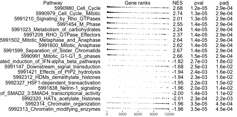
Since the genes were ranked according to their differential expression significance and fold change, with the most significantly down-regulated genes at the top and up-regulated genes at the bottom of the list, the enriched gene sets provides us with some idea of the function of these genes. For example, exampleRanks was generated by testing regulatory T cells against T helper cells, so the enriched pathways may suggest differences between these two types of cells.

Reactome

You can also use Reactome pathways with fgsea. Make sure you have the database installed.

## try http:// if https:// URLs are not supported
source("https://bioconductor.org/biocLite.R")
biocLite("reactome.db")

We'll perform the same analysis as before but this time we'll use the pathways from the Reactome database.

my_pathways <- reactomePathways(names(exampleRanks))

# Reactome pathways have a median of 11 genes
summary(sapply(my_pathways, length))
   Min. 1st Qu.  Median    Mean 3rd Qu.    Max. 
    1.0     4.0    11.0    30.3    30.0  1140.0

fgsea_reactome <- fgsea(pathways = my_pathways, 
                        stats = exampleRanks,
                        minSize=15,
                        maxSize=500,
                        nperm=100000)

head(fgsea_reactome[order(pval), ])
                    pathway         pval         padj        ES      NES nMoreExtreme size
1:               Cell Cycle 1.215983e-05 0.0002401877 0.5469310 2.735403            0  393
2:      Cell Cycle, Mitotic 1.241111e-05 0.0002401877 0.5570318 2.754600            0  346
3: Neutrophil degranulation 1.264302e-05 0.0002401877 0.4305249 2.103791            0  306
4: Signaling by Rho GTPases 1.303169e-05 0.0002401877 0.4151348 1.985009            0  248
5:                  M Phase 1.307497e-05 0.0002401877 0.5080161 2.422413            0  242
6:   Cell Cycle Checkpoints 1.344737e-05 0.0002401877 0.6158766 2.872592            0  200
                               leadingEdge
1:   66336,66977,15366,12442,107995,66442,
2:   66336,66977,15366,12442,107995,66442,
3:    11676,14190,53381,12306,20430,12505,
4: 66336,66977,20430,104215,233406,107995,
5:   66336,66977,12442,107995,66442,52276,
6:   66336,66977,12442,107995,66442,12428,

sum(fgsea_reactome[, padj < 0.01])
[1] 105

Leading edge

Again from the original paper:

Often it is useful to extract the core members of high scoring gene sets that contribute to the enrichment score. We define the leading-edge subset to be those genes in the gene set S that appear in the ranked list L at, or before, the point where the running sum reaches its maximum deviation from zero.

As you may have noticed from the previous section, one of the results column was named "leadingEdge"; this contains the genes that contributed to the enrichment score. I'll use the GSEA performed using the Reactome pathways to illustrate.

# the most significant pathway
fgsea_reactome[order(pval),][1,]
      pathway         pval         padj       ES      NES nMoreExtreme size
1: Cell Cycle 1.215983e-05 0.0002401877 0.546931 2.735403            0  393
                             leadingEdge
1: 66336,66977,15366,12442,107995,66442,

# list of Entrez gene IDs that contributed to the enrichment score
fgsea_reactome[order(pval),][1,]$leadingEdge
[[1]]
  [1] "66336"  "66977"  "15366"  "12442"  "107995" "66442"  "12571"  "12428"  "52276"  "54392" 
 [11] "66311"  "215387" "67629"  "54124"  "12649"  "72415"  "56150"  "57441"  "20877"  "67121" 
 [21] "12615"  "11799"  "66468"  "67849"  "19053"  "73804"  "76044"  "20878"  "15270"  "13555" 
 [31] "60411"  "12580"  "17219"  "69270"  "12575"  "69263"  "12448"  "14211"  "20873"  "18005" 
 [41] "72119"  "71988"  "12189"  "17215"  "12534"  "66156"  "208628" "237911" "22390"  "68240" 
 [51] "228421" "68014"  "269582" "19348"  "12236"  "72151"  "18817"  "21781"  "18968"  "217653"
 [61] "66934"  "272551" "227613" "67141"  "68612"  "68298"  "108000" "23834"  "106344" "56452" 
 [71] "242705" "18141"  "223921" "26886"  "13557"  "26909"  "72787"  "268697" "72155"  "56371" 
 [81] "17535"  "107823" "12531"  "327762" "12567"  "229841" "67052"  "16319"  "66634"  "26931" 
 [91] "67203"  "12235"  "19891"  "74470"  "72083"  "381318" "66570"  "17216"  "19687"  "17218" 
[101] "102920" "29870"  "18973"  "16881"  "17463"  "75786"  "19645"  "19075"  "26417"  "69736" 
[111] "19357"  "76816"  "70385"  "70645"  "22628"  "225182" "22627"  "52683"  "19076"  "18972" 
[121] "231863" "26932"  "12544"  "17997"  "26440"  "68549"  "19088"  "269113" "26444"  "19324" 
[131] "103733" "59001"  "107976" "19179"  "12579"  "232987" "17420"  "228769" "219072" "26445" 
[141] "105988" "69745"  "18538"  "69928"  "11651"  "235559" "68097"  "57296"  "14235"  "19170" 
[151] "17246"  "17220"  "12144"  "50793"  "18392"  "236930" "67151"  "70024"  "59126"  "66296" 
[161] "109145" "71819"  "67733"  "50883"  "12447"  "75430"  "12532"  "14156"  "26442"  "19177" 
[171] "230376" "245688"

# how many genes are in the leading edge?
length(fgsea_reactome[order(pval),][1,]$leadingEdge[[1]])
[1] 172

# how many genes are in the Cell Cycle pathway?
length(my_pathways[['Cell Cycle']])
[1] 393

Summary

The Gene Set Enrichment Analysis (GSEA) has been around since 2005 and has become a routine analysis step in gene expression analyses. It differs from Gene Ontology enrichment analysis in that it considers all genes in contrast to taking only significantly differentially expressed genes. The fgsea package allows one to conduct a pre-ranked GSEA in R, which is one approach in a GSEA. A p-value is estimated by permuting the genes in a gene set, which leads to randomly assigned gene sets of the same size. Note that "This approach is not strictly accurate because it ignores gene-gene correlations and will overestimate the significance levels and may lead to false positives." However, it is still useful in getting an idea of the potential roles of the genes that are up- and down-regulated. If your pre-ranked GSEA returns no significant gene sets, you may still get an idea of what roles the up- and down-regulated genes may be involved in by examining the leading edge set. This set indicates the genes that contributed to the enrichment score.

The example ranks in the fgsea package were ranked on the moderated t-statistic. Another metric that you may consider is to simply take the signed fold change and multiply it by the -log₁₀p-value. For example, if you performed your differential expression analysis with edgeR, you can simply multiply the signed fold change column to the -log₁₀p-value column. This metric is based on this paper: Rank-rank hypergeometric overlap: identification of statistically significant overlap between gene-expression signatures.

Appendix

The author of fgsea provides the R script for generating exampleRanks; for convenience the code is provided below.

source("https://raw.githubusercontent.com/assaron/r-utils/master/R/exprs.R")
gse14308 <- getGEO("GSE14308")[[1]]
pData(gse14308)$condition <- sub("-.*$", "", gse14308$title)
es <- collapseBy(gse14308, fData(gse14308)$ENTREZ_GENE_ID, FUN=median)
es <- es[!grepl("///", rownames(es)), ]
es <- es[rownames(es) != "", ]
exprs(es) <- normalizeBetweenArrays(log2(exprs(es)+1), method="quantile")
es.design <- model.matrix(~0+condition, data=pData(es))
fit <- lmFit(es, es.design)
fit2 <- contrasts.fit(fit, makeContrasts(conditionTh1-conditionNaive,
                                         levels=es.design))
fit2 <- eBayes(fit2)
de <- data.table(topTable(fit2, adjust.method="BH", number=12000, sort.by = "B"), keep.rownames = T)
ranks <- de[order(t), list(rn, t)]

The genes are ranked by the moderated t-statistic, where the sign indicates the fold change

de[order(t), c(1,19:24)]
           rn     logFC   AveExpr         t      P.Value    adj.P.Val        B
    1: 170942 -6.400779 11.670183 -62.22877 5.412495e-11 8.621514e-07 13.91586
    2: 109711 -5.655664 11.107294 -49.47829 2.752658e-10 8.621514e-07 13.15661
    3:  18124 -5.829724  8.730385 -43.40540 6.963327e-10 1.119183e-06 12.62986
    4:  12775 -5.066777 11.472139 -41.16952 1.012754e-09 1.314681e-06 12.39775
    5:  72148 -4.864065  8.365239 -33.23463 4.606844e-09 3.417291e-06 11.34801
   ---                                                                        
11996:  58801  6.730286  9.721764  49.10222 2.905662e-10 8.621514e-07 13.12780
11997:  13730  8.979133  8.379178  50.02863 2.545022e-10 8.621514e-07 13.19797
11998:  15937  5.519076  9.440537  50.29120 2.452293e-10 8.621514e-07 13.21737
11999:  12772  8.833193  9.721834  50.52651 2.372453e-10 8.621514e-07 13.23458
12000:  80876  6.897013 12.040680  52.59930 1.783927e-10 8.621514e-07 13.37922

Visualise the six most significantly down- and up-regulated genes.

library(pheatmap)

my_group <- data.frame(group = pData(es)$condition)
row.names(my_group) <- colnames(exprs(es))

pheatmap(
  mat = es[c(head(de[order(t), 1])$rn, tail(de[order(t), 1])$rn),],
  annotation_col = my_group,
  cluster_rows = FALSE,
  cellwidth=25,
  cellheight=15
)